Showing posts with label epiphany. Show all posts

Sunday, 9 October 2016

Benchmarking Broadcast Strategies

In this post I compare four different strategies to share data between all cores using direct memory writes. I'll evaluate the four strategies using the e_ctimer functions on the epiphany to measure overall execution time and cMesh waits.


Introduction


There are two things I want to look at in this post. Firstly, what performance improvement is available if you try and improve the way you move data around using the cMesh and secondly, how would you measure that improvement.

The reason I'm spending time looking at this is that inter-core communication is the Achilles Heal of distributed memory multi-processors. There are a few algorithms that do not require the cores to share data (known as "embarrassingly parallel") but most do. Given that the whole purpose of using a parallel processing environment is performance, using the best communication strategy is crucial.

To be able to decide which is best, you need to be able to measure it. I used the e_ctimer functions to measure wall-clock performance of four different strategies. To gain some additional insight into what is going on, I used the slightly more complicated eMesh configuration registers to measure the wait times due to mesh traffic.

My conclusion is that, while some small improvements are available by using a carefully thought out strategy, the most important factor is now efficient your algorithm is.

Getting Started


I'm using the COPRTHR-2 beta pre-processor that is available here. At the time of writing it only runs on the Jan 2015 Parallella image.

$ uname -a

Linux parallella 3.14.12-parallella-xilinx-g40a90c3 #1 SMP PREEMPT Fri Jan 23 22:01:51 CET 2015 armv7l armv7l armv7l GNU/Linux

However, while I'm using COPRTHR-2 everything I use is available in COPRTHR-1 and the MPI add-in.

To have a look at the code, use git:

$git clone -b broadcastStrat https://github.com/nickoppen/passing.git 


The Strategies


In my previous post on passing strategies I looked at two broadcast strategies that were essentially the same other than that one had a barrier function on every iteration. It turns out that the barrier function completely dominates the time required by the function. On examination a barrier per iteration was not needed so the non-barrier version was the clear winner. This strategy is my base case.


Base Strategy - "Pass Up"


The base strategy passed all values "up". That is, each core passes the data to the core with a global id one greater than itself looping back to zero when it reached the "last" core with global id equal to fifteen. It stopped when it got back to it's own global id.

Thus, the core with global id 5 would send it's data to the other cores in the following order:

6, 7, 8, 9, 10, 11, 12, 13, 14, 15, 0, 1, 2, 3, 4 and stop because 5 is next.


Refinement 1 - "0 to 15"


I need to do this sort of distribution in my neural network program and when I came to write that routine I thought that the original strategy was a bit complicated. Why not just send the data to the core with global id 0 then 1 then 2 and so on until 15, skipping the local node.

Thus core 5 would send in the following order:

0, 1, 2, 3, 4, skip, 6, 7, 8, 9, 10, 11, 12, 13, 14, 15

I didn't think that this would be a more efficient way to send data but at least the code was simpler.

With both of the preceding strategies, the cores treat the epiphany as if is a linear array of cores. I thought that there might be some improvement by making more use of the vertical, north and south connections between the cores. To this end I came up with two strategies that ignored the artificially linear nature of the global id distribution.


Refinement 2 - "Random"


There is a handy site that generates random number sequences. I generated sixteen of them and ordered my cores accordingly. I remove the local core address for each core and from there it was simply a matter of iterating through the array of cores. No further thought required.


Refinement 3 - "Mapped"


In the final strategy, I tried to come up with a sending order that would try and reduce the number of cores trying to send data along the same channel at the same time. Thus reducing the number of clashes and therefore the amount of time the cores had to wait.

I used a "nearest first" strategy. Thus direct neighbours get the data first. For core 5:


Then I send to cores that are two hops away:


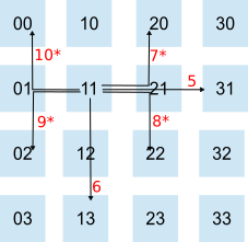
* Note: I have not changed the default "horizontal then vertical" communication strategy employed by the epiphany hardware.

Then, after two hops I do three hops, fours hops etc until all fifteen other cores have received the data. I also vary the initial direction, left first on the top row, then up on the second etc.

Both the "Random" and "Mapped" strategies require a different list of core base addresses for every core. In my kernel all cores get all lists but only use one. If space is tight, these lists could be stored in shared memory and each core would only copy down the list it is going to use. 


The Implementation


Copying


As with my last post on data passing, I use the following to make the copy:

#define NEIGHBOUR_LOC(CORE, STRUCTURE, INDEX, SIZEOFTYPE) (CORE + ((unsigned int)STRUCTURE) + (INDEX * SIZEOFTYPE))

The #define slightly improves the readability in the inner loop:


for (i=firstI; i < lastI; i++)
   *(int *)NEIGHBOUR_LOC(core[coreI], vLocal,  i, (sizeof(int))) = vLocal[i];

The kernel is called 32 times with the amount of data being copied increasing from 1 to 32 integers (ints). The whole loop is repeated 10,000 times to add to the workload and get some more representative numbers.


Clock Timer


The epiphany chip has two timers and they are implemented in hardware (so the best information comes from the Architecture Reference Document not the SDK Reference Document). They count downwards from their initial value.

 The basic usage of a timer is as follows:

e_ctimer_set(E_CTIMER_0, E_CTIMER_MAX);   // set timer register to its max value
start_ticks = e_ctimer_start(E_CTIMER_0, E_CTIMER_CLK); // start the timer to count clock ticks remembering the initial value

// implement the code you want timed 

stop_ticks = e_ctimer_get(E_CTIMER_0);    // remember the final value
e_ctimer_stop(E_CTIMER_0);                // stop timing
time = start_ticks - stop_ticks;          // calculate the elapsed time in ticks

to stop the timer. Again I've #defined these lines:

#define STARTCLOCK0(start_ticks) e_ctimer_set(E_CTIMER_0, E_CTIMER_MAX); start_ticks = e_ctimer_start(E_CTIMER_0, E_CTIMER_CLK);

#define STOPCLOCK0(stop_ticks) stop_ticks = e_ctimer_get(E_CTIMER_0); e_ctimer_stop(E_CTIMER_0);

Note: I've used a C style #define to define an inline function with multiple lines. I've done this to avoid the overhead associated with a function call.


Mesh Timer


The mesh timer is a little more complicated. The start and stop are the same as above but you have to tell the epiphany what mesh event you want to time. You can time wait or access events to the CPU and/or to the four connections (see the MESHCONFIG register definitions in the Architecture Reference). To do this you need to set a value in the E_MESH_CONFIG register. Then, to be neat, you need to restore E_MESH_CONFIG back to what it was before you started.

To initialise the timer to measure all mesh wait ticks:

#define E_MESHEVENT_ANYWAIT1 0x00000200  // Count all wait events

int mesh_reg = e_reg_read(E_REG_MESHCFG);   // make a copy of the previous value
int mesh_reg_timer = mesh_reg & 0xfffff0ff; // blank out bits 8 to 11
mesh_reg_timer = mesh_reg_timer | E_MESHEVENT_ANYWAIT1; // write desired event code in bits 8 to 11

e_reg_write(E_REG_MESHCFG, mesh_reg_timer); // write the new value back to the register

/* Note: the Architecture Reference document (Rev 14.03.11 pp. 148 - 149) seems to imply that bits 4 - 7 control E_CTIMER1 and bits 8 - 11 control E_CTIMER0. This is around the wrong way. Bits 4 - 7 control E_CTIMER0 and bits 8 - 11 control E_CTIMER1. */

Then you start your time as described above but using E_CTIMER_MESH_1 (for E_CTIMER1) and the timer will count the event type you requested.

Stopping is the same as above but then, to be neat you should put the register back to where it was prior to the initialisation:

e_reg_write(E_REG_MESHCFG, mesh_reg); // where mesh_reg is previous value

Again, I've defined inline functions for brevity and performance:

#define PREPAREMESHTIMER1(mesh_reg, event_type)...
#define STARTMESHTIMER1(start_ticks)...
#define STOPMESHTIMER1(stop_ticks)...
#define RESETMESHTIMER1(mesh_reg)...

To make it obvious that I'm using E_CTIMER_0 for the clock and E_CTIMER_1 for the mesh timer I've added a "0" and a "1" onto the end of my inline function calls.

The Results


I plotted the wall clock time of each passing algorithm:


First, let me say that I have NO IDEA why the graph shows time reductions at 9, 17 and 25 integers. Maybe someone who understands the hardware better than me could explain that.

Second, for small amount of data there are some significant gains to be had. The "mapped" strategy outperforms the base line strategy by between 10% to 25% if you are sending 11 integers or less.

Thirdly, as the inner loop comes to dominate the execution time, the difference between the algorithms decreases. Therefore, for larger amounts of data, being really clever in your program delivers increasingly diminishing returns. The 25% difference writing one int shrunk down to about 1% for 32 ints.

Finally, and this is not obvious from the wall clock chart, the improvements in performance come from a more efficient algorithm rather than from better use of the cMesh. As I improved the algorithms I could see the execution time reducing. This is more obvious in the following, somewhat surprising chart:


This chart shows the average number of clock ticks that the cores have to wait for all mesh events. If the reduction in execution time was due to a more efficient use of the cMesh then you would expect that the best performers ("Mapped" and "Random") would be waiting less than the other two strategies.

It seems that the outer loop with fewer iterations is faster at pumping out data into the mesh which is therefore more clogged. However, the increase in waiting time of the "Mapped" strategy was only 6% of the total execution time compared to 4.2% for "Pass Up" and "0 to 15". Thus the difference made a small contribution to the convergence of the strategies as the volume of data increased.

I must also add that the steady upwards trend shown in the above graph is somewhat over simplified. Initially I used 1,000 iterations. That showed the same trend but the lines jumped around all over the place. If you are measuring something that is only a small chuck of the total execution time (in this case, 4% - 6%) and something that is influenced by other factors (i.e. other core's mesh traffic) you need to repeat the test many many times.


Conclusion


Using the e_ctimer functions is a great way to test out alternative implementations. It is like using a volt meter when developing circuits. However, you may need to run your test many thousands of times to get repeatable, representative results.

The cMesh does a pretty consistent job of delivering the data. If one of the broadcast strategies was inherently better I would expect the performance difference to be maintained and even increase as the amount of data rises. If you use direct memory writes for large amounts of data, simple is probably best.

For low volumes, while some improvement is available by tweaking the delivery process, it is your program that determines the overall performance.


Up Next...


I've briefly touched on DMA transfers is a previous post. I'd like to expand this test out beyond 32 ints and compare direct memory writes with DMA transfers. This will mean getting to understand the contents of e_dma_desc_t and how that all works. 

I will also include mpi_bcast if it is available in the next release of COPRTHR2. Here the big question is whether the coordination overhead imposed by MPI is more or less time consuming than using barriers to coordinate the cores.

Saturday, 16 January 2016

Eclipse Part 2 - Host Debugging with the Runtime Environment

Using the Eclipse Run Time Environment


As a followup to my post about compiling on Eclipse I had a quick look at how to use the Eclipse runtime environment. This his handy for debugging host code running on the ARM chip.

I am currently using the 2015.1 Ubuntu version running on a Parallella server. The OpenCL version is 1.6.2. If you want some source code to practice on, use the mandelbrot example from the first Eclipse post.


Preliminaries


For this post I'm assuming that you have a program in Eclipse that has successfully compiled. The steps in the first Eclipse post are still correct for the 2015.1 version of Ubuntu.

I'm still using the JIT compiler because I have not yet figured out a way of using two different compilers in Eclipse. Code::Blocks lets you create different compile targets using different compilers and then combine the results at link time. If there are any gurus out there who know how to do this using Eclipse then please let me know.


Setting Up


The most important thing you need to do before you can run a program is to set up your environment. Eclipse has a runtime environment but it does not pick up critical bits that you need to use the JIT compiler and run your OpenCL application.

Here is what you need to do with a few other bits thrown in:

Choose Properties from the Project menu giving you this dialog:


Click the "Run/Debug Setting" entry on the list and you will see a default Launch configuration. Click Edit to show:


This dialog controls what and how your application is launched from within Eclipse.

The Name: defaults to you project name but in this box it refers to a specific launch configuration. You can have as many as you like to test out different combinations of settings.

I usually leave the other fields as they are because I'm using it to debug and that's what you get as a default. I might disable auto build if it gets annoying.

To get the program running you need the Environment tab.


This is where you set your environment variables. The minimum you will need are LD_LIBRARY_PATH and PATH. 

To add a new variable click the New... button. 

LD_LIBRARY_PATH you can copy from your environment and paste into the New... box as is. 

Do the same with PATH but add :/bin to the end of it. Oddly this is not on your path and is not in Eclipse either and without it, basic stuff like the cp command (needed by the JIT compiler) will not work.

If your program needs any other environment variables include them here also (except PWD - see below).

While we are here, have a look at the Arguments tab:


If your program uses command line arguments type them in the box exactly as you would on the command line. They will appear in argv as per normal.

If you want to change the working directory, un-click the Use Default box and type the directory you want in the text box. This stands in for the PWD variable. Note that Eclipse will not know what $HOME is unless you have included it as an environment variable in the Environment tab.


Running


Now that you have set the environment you can run your program from the tool bar:


The green Play icon has a small downwards pointing arrow next to it. Your run time configurations will appear on the on the top of the list. Click the one you want to use or just press the icon if you only have one.

This will run your program using the console sub-window for text output.


Debugging


Notice the little insect on the tool bar next to the play button. This launches a debug session which uses the same configurations that you defined previously except it takes notice of break points. Set break points using the Run menu:


Press the creepy-crawly button to launch the debug session. This will pop up a perspective switch warning:


Just press "Remember my decision" and Yes never to be annoyed by this again.

Then you will see the full glory of the debug window:


There is more here then this short tutorial can cover and I cannot say that I'm in any way an expert. Underlying the fancy windows is gdb which I find annoying and so I know the minimum I need to know to figure out what is going wrong.

The usual navigation buttons are next to the Resume button and the in-scope variables are in the top right window. For some reason, variables are often "optimized out" which is frustrating.


Finally


I still have not made any progress with kernel debugging on the Epiphany. If I do, I'll let you know.

For now, have fun and write brilliant code.

Sunday, 6 December 2015

Getting It Done - What I learnt from finishing the Neural Network Algorithm

Sometimes, implementation causes rethinks. In this post I'll review the design decisions I've made getting the back propagation algorithm working, hopefully shedding some light on the practicalities of implementing an algorithm using the Parallella architecture that may be helpful to others.

Before reading this post, I highly recommend watching the presentation by Anish Varghese from the ANU. They did some tricky stuff in machine code to gain a performance boost that is not available in straight OpenCL but their comments on the relative speed of inter-core communication and ARM-Epiphany communication is relevant regardless of language. 

Writing this post I'm using Brown Deer OpenCL (version 1.6.2) and the Ubuntu 14.04 image from 30 Jan 2015.

To have a look at the code referred to in this post look here or execute the following shell command:

git clone -b blog12Files https://github.com/nickoppen/nnP.git


Introduction


Since the last posting, I have written the code that trains my neural network - a process called back propagation. The first thing I had to do was to restructure the feed forward kernel so that it did not discard the intermediate values that are needed in the backward pass. However, it was the management of the complexity that proved the biggest challenge. To manage the complexity I made two design decisions one of which worked out and one that didn't.

Restructure of Feed Forward


My primary goal was to get the algorithm working correctly with speed and efficiency in second place. I had already written the first part of the process (called the feed forward pass) and I'd made some design decisions that were suitable for that process in isolation but proved poor choices for back propagation. 

A neural network is made up of a number of layers (>=3). Each layer takes an input vector and produces an output vector which then become the input to the next layer. When only running the network forward the intermediate results can be discarded and initially that is what I did.

However, when I came to write the back propagation process, I needed these values. I had to change the feed forward algorithm to keep them. While I think I came up with a better solution in the end, the basic lesson, "start with the end in mind" aka "Top down design" still applies.


Complexity - Sometimes you can make it worse!


Back propagation is a tricky little algorithm. Adjusting the weights requires calculating the error in the output and for the intermediate layers that is a sum of the errors on the outgoing weights. In a single threaded implementation you just take one (intermediate) node at a time and iterate through the outgoing weights which are all available in shared memory, calculate the error and then iterate through the incoming weights and calculate the adjustment. While this is a little simplified, the key point is that all of the data is available at all times. 

In the Epiphany architecture each processor has its own memory and so how the task is split up and how data is shared between processors are critical design decisions and come with their own set of problems.

Decision 1 - What goes where


In my first blog post I discussed carving up the task. It was a very "thinking about" sort of post. It had to be, I hadn't gotten the Parallella yet. For the purposes of this post, I'll take a simpler approach. EVERY CORE GETS 1/16th OF THE JOB (or as close to it as possible).

Complexity 1: Indexes

That does not sound complicated but even in a simple, input -> process -> output where you are processing data in arrays you start to get a proliferation of indexes. For example:


You have one for the global input, one for the local copy of the chunk processed by the individual core from which you produce a chunk of output which you then have to copy back to global memory before exiting. If the dimensions of the input and output are different this means that you are juggling four indexes.

A neural network is a little more complicated still. They are multi-dimensional with the size of each dimension (i.e. each layer) changing as you pass through the data structure.

Complexity Reducing Idea No. 1: Keep all the arrays the same size. Therefore the data structure private to the core is the same size as the global arrays. You have to make is as big as the biggest layer and then recalculate where each core starts and stops as you pass through the data. The data flow would look like this (highly simplified):


Clearly there is wasted space in the memory local to all cores (where space is at a premium) but traversing all arrays needs only one index.

Initially I had the global input and the local copy of the input aligned and the local copy of the node biases aligned and the intermediate values and the output aligned. That worked while I was only running the network forward. Then I got to do the back propagation and remembered that I needed to keep the intermediate values generated by the hidden layers. Then I decided that it would be a good idea to keep a copy of the node biases (and weights) so that they could be updated locally and the training could be run multiple times. Then I decided that it would be more efficient for the input to be copied onto the front of the array containing the output for each layer then it could be treated in the same way as the output from layer zero.

Idea No.1 turned out to be not very bright at all. Now I have virtually no alignment and a lot more wasted space that I bargained for - none of the benefit and a much higher cost. The other thing about back propagation is that you are referring to values from the current layer, the next layer and the previous layer in order to adjust the weights so you end up with lots of indexes anyway. This mess is still a part of the files for this post. I'll clean it up for the next version.

The only solution as I see it is to minimise the use of private memory and use descriptive names for the indexes. Coming up with good names is tedious and difficult but in a complex program it will make a huge difference. You will also end up with a lot of "parallel" indexes in for loops, thus: 

local_index = global_start - core_offset;   // set the relative start positions
for (global_array_iterator = global_start; global_array_iterator < global_end; global_array_iterator++)
{
     local_array[local_index] = genius(global_array[global_array_iterator]);
     local_index++;    // manually advance one iterator
}

Also, using the overall strategy of copy-in, process, copy-out will mean that mixing the local (_private) memory indexes and the global memory indexes are not mixed too much.

I store all of the indexes in an array of structures so that I don't have to work it out each time. This meant that there was an array of indexes that needed its own index but that came for free because it was the same as the layer that I was working on (i.e. the outermost for loop index).

Decision 2: Passing Intermediate Values


So, each core is processing 1/16th of the data. In my neural network simulator I decided that the variable length data is passed in via a couple of arrays and that the space for them is compiled into the kernel using JIT compilation as I described in a previous post. The method I used to decide which core processed which section of the data was as follows:

#define CORECOUNT 16

int gid = get_global_id(0);
int allCores = dataWidth / CORECOUNT;  /// all cores get this many
int leftOver = dataWidth % CORECOUNT;  /// the remainder are distributed one per core starting from core0 until all are allocated

int start = ((gid * allCores) + min(gid, leftOver)); 
int end = start + allCores + ((gid < leftOver) ? 1 : 0);

This works well for each core to determine where to start processing in the global data structure. What it does not tell you is which core is processing an arbitrary data point. 

If you have read my hand-waving description of the back propagation process you will recall that the "back" part refers to the backwards flow of data to previous layers in order to determine the error of those layers (let's call this data "weight deltas"). 

I've arranged my weights to be contiguous for the node that receives their contribution in the forward pass. This allows the forward pass to calculate the node value by traversing a contiguous sequence of weight values. In the backwards pass the weight delta of each weight has to be returned to its "origin node". To pass it directly back to the core that "owns" that node I needed a similar simple formula.

Complexity 2: Inter-core communication

With processing distributed over a number of cores, figuring out what core is responsible for which datum can be difficult.

Complexity Reducing Idea No. 2: Use global memory as a scratch pad to communicate between the cores.

The good thing about global memory is that it is big (32Mb). The bad thing is that it is slow. The ugly thing is that all cores have equal access to all of it and therefore you'd better be careful about race conditions.

To return the weight delta to it's "origin node", I calculate it when updating "destination node" and write it to the global array called g_weightDeltas. Then, when I come to calculate the error of the "origin node" I read it from g_weightDeltas adding them as I go. This is not quite as simple as it sounds. When calculating the error of each "origin node" you need a weight delta from all nodes in the subsequent layer. I decided to organise g_weightDeltas in the same way is the weights themselves for consistency. This means that writing them happens in the same order as calculating them but reading them requires some index gymnastics to pick the right value from the array, thus:

outputError += g_weightDeltas[nextLayer_globalWgtZero + (w * curLayerWidth) + layerNodeIterator];

where:
outputError is the accumulated error for the node
nextLayer_globalWgtZero is the index of first weight connecting the current layer with the next layer (don't forget that I'm organising the weight deltas in the same way as the weights)
curLayerWidth is the number of nodes in the current layer (therefore the number of weights for each node in the next layer)
w is the current weight
layerNodeIterator is the current node

Idea No. 2 did work out. For a little index gymnastics I saved a bit of tricky programming (aka laborious debugging) and I now have a way of checking the inter-core communication when I come to do it (leaving the global array there for now I can check the directly passed values to the global array values). The global array is easy to debug because I can call clmsync on return and check it's values. 

For this stage of the project, I'm not really concerned about speed but I will have to address this in the next version. I avoid race conditions in a macro way by ensuring that every layer has updated itself and the global array before the global array is read by using a barrier command. 

There is one little issue to remember when using global memory for internal purposes. It needs to be declared and allocated on the host. You don't need to do anything with it on the host but it cannot be allocated in a kernel.


Looking Forward


Having (yet again) learnt to design before coding, I've had a think about how I want the overall system to look. 

In my value passing experiment, I noticed that the overhead of launching a kernel is huge. Therefore the best way of getting the most performance out of the Epiphany is to launch the kernel once and then keep feeding it with data until there is not more data left.

This suits back propagation well because training requires multiple iterations through the training set which could be too big for global memory. Also, loading it into global memory before launching the kernel would introduce a serial component to the process that could be done by the host in parallel with the training that is happening on the Epiphany (and that's what we are all about after all).

Multiple executions of the feed forward algorithm also makes sense in certain applications. If you are using the neural net to recognise features in a video stream you will probably want to pass frames to the network as they arrive. Waiting for the kernel to launch for each frame would probably cause frame to be dropped while the host waits.

So, my target system looks like this:


It looks a bit complicated but the key thing to get is that the host is reading the next lot of input data into global memory while the Epiphany is processing. It then uses some sort of signalling mechanism to indicate that the data is ready. When the Epiphany is done, it signals back to the result reader thread to pull back the results from global memory.

To simplify the diagram, I've assumed that the main host thread is always going to be slower than the Epiphany and therefore never has to wait. While this might be the case in some applications, it may also have to wait to ensure that it does not get too far ahead and starts over-writing unprocessed data.


Up Next...


The next job is to figure out how to do the signalling. I'm going to have a look at the MPI libraries now included in the Brown Deer system. I think that they will do the job. 

After that, I'll tighten up local memory and figure out how to pass the weight deltas back to their origin node in an efficient manner.

As always, please comment, especially if I've missed something or if you have a suggestion. You can comment either here on Blogger, on the Parallella forum or on reddit.

Friday, 27 March 2015

Intercore Communication and Profiling (sort of...)

In this post I will describe three ways of passing data between cores and provide some empirical comparisons using a rudimentary method of profiling.


In my last post I described a method of passing data from one core to the others using a broadcast strategy. Each core calculated the base address of each other core and wrote to a data structure at a known address. At the time I wrote my last post, I believed that this is could be improved and made a little more programmer friendly. To test out some alternative data passing methods, I designed a little experiment and used a rudimentary profiling strategy. I did find a significantly better alternative, but not where I expected.

Writing this post I'm using Brown Deer OpenCL (version 1.6) and the original Ubuntu 14.04 image.


To get my sample code execute:

git clone -b blog10files https://github.com/nickoppen/passing.git


Profiling in OpenCL


OpenCL provides the cl_event structure to pass onto the execution queue, created with the CL_QUEUE_PROFILING_ENABLED flag set to allow timing information to be retrieved using the clGetEventProfilingInfo call. This seems pretty straight forward but unfortunately this is currently not supported (according to the Parallella Quick Start Guide).

This leaves us with the timing support provided by C++. The library <ctime> provides the calls time(time_t & time) and clock_t clock = clock(). The time() call returns the number of seconds since 1 Jan 1970 which is too coarse to measure the execution of a small kernel. The clock() call returns the number of system clock ticks which is much smaller time intervals and, if all of the profiling is done on the same machine, will be accurate enough to get a feel for comparative execution times.

Surrounding the forka call time stamps seems simple enough but one must remember that the command queue is asynchronous so any calls prior to the forka and the forka itself must be called with the flag CL_EVENT_WAIT.

#include <ctime>

clock_t tstart, tend;


clmsync(stdacc, 0, debug, CL_MEM_DEVICE|CL_EVENT_WAIT);

tstart = clock();
clforka(stdacc, 0, krn, &ndr, CL_EVENT_WAIT, n, 1, debug);
tend = clock();

The main problem with this approach is that it measures everything that the forka does. Have a look at Adam Taylor's host code for a simple "Hello, World!" application. There is a lot of setting up code, which is buried within the forka. This is a little clumsy but will have to do for now.


Intercore Value Passing


Core ID Abstraction


In my last post I used the little gem (from djm):

#define LOCAL_MEM_ADDRESS_BASE(gid) (((32 + ((gid) / 4)) << 26) | ((8 + ((gid) % 4)) << 20))

to calculate the base address of the core and then used:

*(float *)(LOCAL_MEM_ADDRESS_BASE(gid_next) + ((unsigned int) derived) + (index * sizeof(float))) = value_being_passed;

Now, I love bit shifting as much as the next programmer but I don't really have to work out what every base address is. If I know my global id ( gid = get_global_id() ) I can figure out where the executing core is in the mesh and its relationship with all other cores because the base addresses don't change.

My second love is hexadecimal memory locations but they really increase your nerd status when your wife or girlfriend looks over your shoulder and wonders what on earth you are doing late into the night. Seriously though, does 0x8080 really mean anything to you? And what is it's relationship with 0x84b0. How many hops are there between the two?

The eSDK has a way of partitioning the cores based on their location in the grid. The stdcl library does not support this but it is still a good idea. Instead of 0x8080 we could say core00 and then it is obvious that there are 5 hops to core31 (formerly known as 0x84b0).

That suggests to me that the first snippet above (although pure poetry) can be abstracted away into some nice, convenient and most importantly, efficient include file that looks like this:

#define core00 0x80800000
#define core10 0x80900000
#define core20 0x80a00000

...


Topology Abstraction


The Epiphany is a rectangular mesh with each core connected to its nearest neighbours. This is great, but what if your application is better suited to a ring structure where it only had to communicate with two cores on each side of it in the ring. For this application, it would be convenient to relate to the next core as NEXT and the previous core as PREV. In this case, the ring topology would look like this:


If data only needed to flow around in one direction, then you would only need to refer to NEXT.

Similarly, you could define a row topology:


Or, if you really did need 3 Dimensional processing, a mesh topology where you only had to refer to NORTH, SOUTH, EAST and WEST would be really handy:


In the row and grid topology, the ends (e.g. RIGHT of core00) get assigned 0x0.

I have implemented these three topologies and used the ring in my sample code. The relevant code is:

unsigned int NEXT, PREV, ringIndex, gidOrder[CORECOUNT];
...
initRing(&NEXT, &PREV, &ringIndex, gidOrder);


The initRing call initialises all of the variables which are:
  • NEXT: the next core base address in the ring
  • PREV: the previous core base address in the ring
  • ringIndex: the position of the executing core within the ring (core00 is assigned 0 and core01 is 15)
  • gidOrder: an array with the global_ids in the order in which they come in the ring (gidOrder[ringIndex] == get_global_id(0)


Such definitions would even abstract away most of the need to refer to coreXX and would mean that, once set up, no core would have to execute an if... else... to figure out where it is in the mesh. The only exception would be using the row and mesh topologies, the code would have to check that it is not on the edge with no core further down the chain.

Abstracting the Assignment


One final abstraction is to clean up the assignment. To this end I've defined:

#define NEIGHBOUR_LOC(CORE, STRUCTURE, INDEX, SIZEOFTYPE) (CORE + ((unsigned int)STRUCTURE) + (INDEX * SIZEOFTYPE))
#define NEIGHBOR_LOC(CORE, STRUCTURE, INDEX, SIZEOFTYPE) (CORE + ((unsigned int)STRUCTURE) + (INDEX * SIZEOFTYPE))

(The only difference between the two is the spelling of neighbour/neighbor.) 

Which is used (for an int assignment):

*(int*)NEIGHBOUR_LOC(NEXT, vLocal, i, sizeof(int)) = vLocal[i];

I still find this a bit clumsy but better than the original.

The Passing Experiment


The whole point of this exercise was to see if I could find a better alternative to the core-to-core broadcast method I implemented in my feed-forward pass of my neural network.

(For those who don't want to wade through my first post, the feed-forward pass is a series of matrix multiplication steps where the task is split between all cores. Each step produces another matrix which then is one input of the next step. Every core needs all of the values produced in the previous step, therefore every core must pass its results to every other core.)

The Original Method - Broadcast


The original method iterated through every remote core and wrote directly into it's memory. The code was simple enough but my "back of the envelope" calculation estimated that if every core just sent one value, there would be 640 intercore hops in the whole process.

I did improve on the original a little. I only calculated the remote core's base ID once (rather than every time I sent a value which is a obviously a waste of time).

Alternative Zero - Broadcast No Wait


I was also pretty sure that I didn't need so many calls to barrier() given that each core "owned" a chunk of the storage array on all cores and it alone wrote to it. So my first change was to implement the same broadcast strategy but with no barriers.

I wanted to write the best kernel I could so I generated an array of all core IDs (core00... core33) and iterated through the array sending all values to it except when the destination core ID was the same as the local core ID (no point in sending the value to itself).

Then I came up with two alternative strategies to test using my ring topology described above.

Alternative One - Unicast


Unicast uses the ring topology and passes it's local values to the next core. Then, it passes the values it has just received from the previous core in the ring onto the next core and so on until all values have flowed around the ring.

This would minimise the number of clashes but it does not use very much of the available bandwidth. Hence:


Alternative Two - Multicast


I read somewhere that the Epiphany has two channels on the cMesh (used for intercore write messages). Multicast (which should really be called Bicast) again uses the ring topology but passes values in two directions, thereby using both channels. Like Unicast, it first sends its own values (but in both directions) and then sends the values it has just received from its neighbours - values received from PREV are passed onto NEXT and values received from NEXT are passed onto PREV).


The Results


To see some sort of sensitivity I called each method 16 times. Each call I incremented an argument (n) from 1 to 16. All kernels passed n values to its neighbours. I expected to see some difference in execution time based on the kernels algorithm and some sort of trend line as n increased. However, my initial experiment did not show any difference between the methods or the volume of data passed at all. The chart looked like this:


The Y-axis is the number of clock ticks per call and the X-axis has the passing method (broardcast, broadcast No Wait, multicast and unicast), in ascending order of the number of values passed.

This was a bit disappointing at first. Taking into account a bit of random scatter, all the methods looked the same and there was no discernible trend line based on n. The average for all methods was just over 119,000 ticks. I thought I should take a larger sample.

At first, I surrounded everything in a loop and ran it 100 times. This made hardly any difference at all. The average nudged up a time bit but the overall picture looked the same.

As I mentioned above, the timing method I used measured the whole of the forka call. Because there was so little change between 1  and 100 iterations, I can only assume that the 119,000 odd clock ticks were all overhead!

Clearly, to see any sort of difference I'd have to dramatically increase the workload. So... 100,000 iterations...


Finally, a data set that tells a story! The averages (which include the 119,000 tick loading time) were:


  • Broadcast: 2,545,798 ticks
  • Broadcast No Wait: 302,535 ticks
  • Multicast: 1,521,429 ticks
  • Unicast: 2,623,446 ticks
And a roughly steady increase with the amount of data being sent.


But hang on... what story does it tell?


I was completely amazed by this result. Getting rid of the calls to barrier() decreased the execution time by almost 90%! Sure the algorithm was a little better but not that much!

Similarly, Multicast, with almost half the calls to barrier(), ran in almost half the time.

Here I was thinking that the number of hops was the dominant time consumer!

Conclusions


From this experiment, I propose the following conclusions:


0. Don't Wait... Minimise the use of barrier()


Coordinating cores using calls to barrier() is expensive.

While I thought my fancy topologies would speed things up by reducing the number of hops, the algorithm needed the cores to coordinate. In a "pass-it-along" scenario, each core had to make sure that the cores around it had successfully delivered their value(s) before it could pass it (or them) along.

Broadcast, using point-to-point communication didn't need coordination so the extra transmission cost was insignificant.

1. Give your cores a lot of work to do. 


The thing that slows parallel architectures down in general and especially with distributed memory architectures is communication overhead. This is usually interpreted as, "The cores need to pass information between each other and wait for results". However, when working with a remote device, communication overhead includes the amount of time the main processor needs to send the accelerator the kernel and the data to work on as well as the intercore communication.

So, when designing your system, cut off as big a chunk of work you can and get the little cores to do as much as possible - they are quite powerful... they can handle it.


Final thought...


While my topologies didn't deliver any significant gain in this case, I think that they would still be useful if the topology suited the algorithm. If I come across one, I'll write another post.


Up Next


I'm going to upgrade my system to the new image. I believe that the reboot is more reliable and you don't need to run you programs as root. Not a big deal but I still forget to login using su every now and then. I'll also revisit my old posts to update them if need be.

Then I'll keep going on my neural network simulator... Stay tuned.